Page 310 - How To Implement Lean Manufacturing

An Experiment in Variation, Dependent Events, and Inventory 287

teams will average 21, but their factory simulations will perform differently because …
well, let’s do the experiment.
Creating the Data
1. Roll the dice (or die) and count the total spots.
2. Multiply the total by the multiplier for your team.
3. Enter this number in the oval on the plant simulation spreadsheet, starting with
Cycle 1, station 1.
4. Repeat steps 1 thru 3 for Cycle 1, station 2, and so on, through Cycle 1,
station 8 ...
5. Do this for 20 cycles at least, which means several copies of the spreadsheet will
be needed.
6. To simulate the process, fill in the rectangles, described in this chapter in the
section entitled, “Processing the Data.”
7. Calculate the production.
8. Sum the totals, as in the summary data table shown in Table 18-2.

Processing the Data
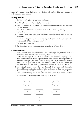
1. Each horizontal row of information is a cycle for this process, and each cycle of
production goes through eight processing steps.
The oval (see Figs. 18-1 and 18-2) represents the instantaneous capacity of that
work station based on station capacity alone. Since each die has the potential of
numbers 1 through 6, for Team 1 since its multiplier is six, it can be seen that the
instantaneous capacity for each station is a value from 6 to 36. And in the high
variability case of 1 die, the only possible values are 6, 12, 18, 24, 30, and 36.
2. The rectangle directly below the oval, Rectangle 1, is the amount of material
(think of them as kits) that is available for the next station in the cycle. We assume
the warehouse has infinite material, so there is no material constraint at the first
station. The following then becomes the two possible constraints on the system:
a. Instantaneous Station capacity given by the dice data

1 2 3

4

FIGURE 18-1 The data format for the experiment.