Page 71 - Human Inspired Dexterity in Robotic Manipulation

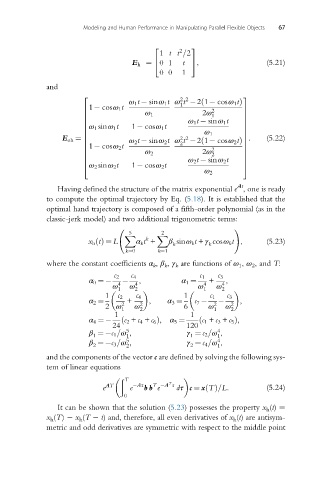
Modeling and Human Performance in Manipulating Parallel Flexible Objects 67

2 2 3
1 tt =2
E h ¼ 01 t 5 , (5.21)
4
00 1
and
2 2
2 3
ω 1 t sinω 1 t ω t 2ð1 cosω 1 tÞ
1
1 cosω 1 t
6 2ω 2 7
ω 1 1
6 7
ω 1 t sinω 1 t
6 7
6 ω 1 sinω 1 t 1 cosω 1 t 7
6 7
ω 1
2 2 7: (5.22)
6 7
E oh ¼ 6 ω 2 t sinω 2 t ω t 2ð1 cosω 2 tÞ
2
6 1 cosω 2 t 7
6 2ω 2 7
ω 2
6 2 7
6 ω 2 t sinω 2 t 7
4 ω 2 sinω 2 t 1 cosω 2 t 5
ω 2
At
Having defined the structure of the matrix exponential e , one is ready
to compute the optimal trajectory by Eq. (5.18). It is established that the
optimal hand trajectory is composed of a fifth-order polynomial (as in the
classic-jerk model) and two additional trigonometric terms:
!
5 2
X k X
x h ðtÞ¼ L α k t + β sinω k t + γ cosω k t , (5.23)
k k
k¼0 k¼1
where the constant coefficients α k , β k , γ k are functions of ω 1 , ω 2 , and T:
c 2 c 4 c 1 c 3
α 0 ¼ , α 1 ¼ + ,
ω 4 1 ω 4 ω 4 1 ω 4 2
2
1 c 2 c 4 1 c 1 c 3
α 2 ¼ + , α 3 ¼ c 7 ,
2 ω 2 1 ω 2 2 6 ω 2 1 ω 2 2
1 1
α 4 ¼ ð c 2 + c 4 + c 6 Þ, α 5 ¼ ð c 1 + c 3 + c 5 Þ,
24 120
5
4
β ¼ c 1 =ω , γ ¼ c 2 =ω ,
1
1
1
1
5
4
β ¼ c 3 =ω , γ ¼ c 4 =ω ,
2
2
2
1
and the components of the vector c are defined by solving the following sys-
tem of linear equations

ð T
T A τ
e AT e Aτ bb e T dτ c ¼ xðTÞ=L: (5.24)
0
It can be shown that the solution (5.23) possesses the property x h (t) ¼
x h (T) x h (T t) and, therefore, all even derivatives of x h (t) are antisym-
metric and odd derivatives are symmetric with respect to the middle point