Page 76 - Hydrogeology Principles and Practice

HYDC02 12/5/05 5:38 PM Page 59

Physical hydrogeology 59

Examples of analytical solutions to one-dimensional BO X
groundwater flow problems 2.9

To illustrate the basic steps involved in the mathematical analysis of h =− Q ⋅ 0 +
groundwater flow problems, consider the one-dimensional flow 0 Kb c
problem shown in Fig. 1 for a confined aquifer with thickness, b. The
∴ c = h
total flow at any point in the horizontal (x) direction is given by the 0
equation of continuity of flow:
which gives the solution:
Q = q ⋅ b eq. 1
h = h − Q x eq. 5
where q, the flow per unit width (specific discharge), is found from 0 Kb
Darcy’s law:
The specific solution given in equation 5 relates h to location, x, in
terms of two parameters, Q and Kb (transmissivity), and one bound-
q =− K h d eq. 2 ary value, h . The solution is the equation of a straight line and pre-
x d 0
dicts the position of the potentiometric surface as shown in Fig. 1.
Also note, by introducing a new pair of values of x where h is known,
where x increases in the direction of flow. Combining equations 1
for example x = D, h = h , we can use the following equation to
and 2 gives the general differential equation: D
evaluate the parameter combination Q/Kb since:
Q =− Kb h d eq. 3 Q h − h
=
x d 0 D eq. 6
Kb D
By integrating equation 3, it is possible to express the groundwater
If we know Kb, we can find Q, or vice versa.
head, h, in terms of x and Q:
As a further example, the following groundwater flow problem
provides an analytical solution to the situation of a confined aquifer
dh Kb dx receiving constant recharge, or leakage. A conceptualization of the
Q
=−
problem is shown in Fig. 2 and it should be noted that recharge, W,
at the upper boundary of the aquifer is assumed to be constant
∴= − Q x + c eq. 4 everywhere.
h

Kb Between x = 0 and x = L, continuity and flow equations can be
written as:
c is the constant of integration and can be determined by use of a
supplementary equation expressing a known combination of h and Q = W(L − x) eq. 7
x. For example, for the boundary condition x = 0, h = h and by
0
applying this condition to equation 4 gives:

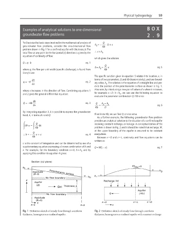
Fig. 1 Definition sketch of steady flow through a uniform Fig. 2 Definition sketch of steady flow through a uniform
thickness, homogeneous confined aquifer. thickness, homogeneous confined aquifer with constant recharge.