Page 77 - Hydrogeology Principles and Practice

HYDC02 12/5/05 5:38 PM Page 60

60 Chapter Two

BO X
Continued
2.9

=
Q Kb h d eq. 8
x d
and between x = L and x = D:
Q = W(x − L) eq. 9

Q =− Kb h d eq. 10
x d

By combining the first pair of equations (eqs 7 and 8) between x = 0
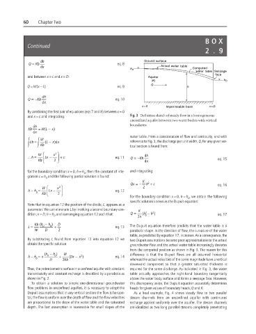
and x = L and integrating: Fig. 3 Definition sketch of steady flow in a homogeneous
unconfined aquifer between two water bodies with vertical
boundaries.
h d
=
−
Kb WL( x)
x d
W L ( x) dx water table. From a consideration of flow and continuity, and with
=
−
reference to Fig. 3, the discharge per unit width, Q, for any given ver-
dh
Kb
tical section is found from:
W ⎛ x 2 ⎞ h d

∴= h ⎜ Lx − ⎟ + c eq. 11 Q =− Kh
Kb ⎝ 2 ⎠ x d eq. 15
for the boundary condition x = 0, h = h , then the constant of inte- and integrating:
0
gration c = h and the following partial solution is found:
0
K
Qx =− h + c eq. 16
2
W ⎛ x ⎞ 2
2
−
−
h h = ⎜ Lx ⎟ eq. 12
0
Kb ⎝ 2 ⎠
For the boundary condition x = 0, h = h , we obtain the following
0
specific solution known as the Dupuit equation:
Note that in equation 12 the position of the divide, L, appears as a
parameter. We can eliminate L by invoking a second boundary con- K
2
dition, x = D, h = h and rearranging equation 12 such that: Q = x 2 ( h − h 2 ) eq. 17
0
D
+
=
L Kb h ( D − h 0 ) D eq. 13 The Dupuit equation therefore predicts that the water table is a
W D 2 parabolic shape. In the direction of flow, the curvature of the water
table, as predicted by equation 17, increases. As a consequence, the
By substituting L found from equation 13 into equation 12 we two Dupuit assumptions become poor approximations to the actual
obtain the specific solution: groundwater flow and the actual water table increasingly deviates
from the computed position as shown in Fig. 3. The reason for this
−
h h = x h ( D − h 0 ) + W ( Dx − x 2 ) eq. 14 difference is that the Dupuit flows are all assumed horizontal
0
D 2 Kb whereas the actual velocities of the same magnitude have a vertical
downward component so that a greater saturated thickness is
Thus, the potentiometric surface in a confined aquifer with constant required for the same discharge. As indicated in Fig. 3, the water
transmissivity and constant recharge is described by a parabola as table actually approaches the right-hand boundary tangentially
shown in Fig. 2. above the water body surface and forms a seepage face. However,
To obtain a solution to simple one-dimensional groundwater this discrepancy aside, the Dupuit equation accurately determines
flow problems in unconfined aquifers, it is necessary to adopt the heads for given values of boundary heads, Q and K.
Dupuit assumptions that in any vertical section the flow is horizon- As a final example, Fig. 4 shows steady flow to two parallel
tal, the flow is uniform over the depth of flow and the flow velocities stream channels from an unconfined aquifer with continuous
are proportional to the slope of the water table and the saturated recharge applied uniformly over the aquifer. The stream channels
depth. The last assumption is reasonable for small slopes of the are idealized as two long parallel streams completely penetrating