Page 105 - Innovations in Intelligent Machines

UAV Path Planning Using Evolutionary Algorithms 95

1

3

angle
1
angle
2
Target
4
2
angle = sort_angle
4 1
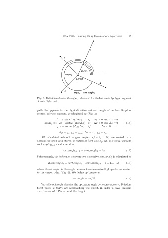
Fig. 3. Definition of azimuth angles, calculated for the last control polygon segment
of each flight path

path the opposite to the flight direction azimuth angle of the last B-Spline
control polygon segment is calculated as (Fig. 3)
⎧
arctan (∆y/∆x) if ∆y ≥ 0 and ∆x ≥ 0
⎨
angle j = 2π − arctan (∆y/∆x) if ∆y< 0 and ∆x ≥ 0 (13)
π + arctan (∆y/∆x) if ∆x< 0
⎩
∆y = y n−1,j − y n,j , ∆x = x n−1,j − x n,j .
All calculated azimuth angles angle ,(j =1,...,N) are sorted in a
j
descending order and stored as variables sort angle . An additional variable
j
sort angle N+1 is calculated as
sort angle N+1 = sort angle 1 − 2π. (14)

Subsequently, the deference between two successive sort angle j is calculated as

∆sort angle j = sort angle j − sort angle j+1 ,j =1,...,N, (15)
where ∆sort angle is the angle between two successive flight paths, connected
j
to the target point (Fig. 4). We define opt angle as
opt angle =2π/N. (16)

Variable opt angle denotes the optimum angle between successive B-Spline
flight paths as UAVs are approaching the target, in order to have uniform
distribution of UAVs around the target.