Page 107 - Innovations in Intelligent Machines

UAV Path Planning Using Evolutionary Algorithms 97
specific time step. Subsequently, the distances between all UAVs are calcu-
lated in each time step and in case that a distance is less than a predefined
safety distance d safe , a penalty is added to term f 4 .
Term f 5 is calculated as
N

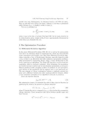
f 5 = (t max −t curr j ) /t max (18)
j=1
where t max is the time of arrival of the last UAV. As the main objective is
to obtain feasible paths, weights in Eq. 10 were experimentally determined in
order term w 2 f 2 dominate the rest.

5 The Optimization Procedure

5.1 Differential Evolution Algorithm

In this work, Differential Evolution (DE) [40, 41] is used as the optimization
tool. DE is an extremely simple to implement EA, which has demonstrated
better convergence performance than other EAs. Differential Evolution algo-
rithm represents a type of Evolutionary Strategy, especially formed in such
a way, so that it can effectively deal with continuous optimization problems,
often encountered in engineering design, being a recent development in the
field of optimization algorithms. The classic DE algorithm evolves a fixed size
population, which is randomly initialized. After initializing the population,
an iterative process is started and at each iteration (generation), a new popu-
lation is produced until a stopping condition is satisfied. At each generation,
each element of the population can be replaced with a new generated one.
The new element is a linear combination between a randomly selected ele-
ment and a difference between two other randomly selected elements. Below
a more analytical description of the algorithm’s structure is presented.
Given an objective function

f obj (X):R n param → R, (19)
the optimization target is to minimize the value of this objective function by
optimizing the values of its parameters (design variables)

,x j ∈ R, (20)
X = x 1 ,x 2 ,...,x n param
where X denotes the vector composed of n param objective function parameters
(design variables). These parameters take values between specific upper and
lower bounds
(L) (U)
x ≤ x j ≤ x ,j =1,...,n param . (21)
j j