Page 106 - Innovations in Intelligent Machines

96 I.K. Nikolos et al.

1

3
Dsort_angle
3

Dsort_angle
4
Dsort_angle
2
Target
4
2 Dsort_angle 1

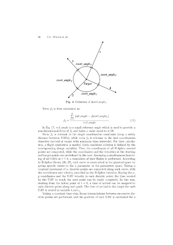
Fig. 4. Definition of ∆sort angle j
Term f 3 is then calculated as:

N
|opt angle − ∆sort angle j |
j=1
f 3 = . (17)
ref angle
In Eq. 17, ref angle is a small reference angle which is used to provide a
non-dimensional form of f 3 and takes a value equal to π/20.
Term f 4 is relevant to the single coordination constraint (keep a safety
distance between UAVs), while term f 5 is relevant to the first coordination
objective (arrival at target with minimum time intervals). For their calcula-
tion, a flight simulation is needed. Each candidate solution is defined by the
corresponding design variables. Then the coordinates of all B-Spline control
points are computed, while the coordinates and the velocities at the starting
and target points are predefined by the user. Assuming a simultaneous launch-
ing of all UAVs at t = 0, a simulation of their flights is performed. According
to B-Spline theory [36, 37], each curve is constructed in the physical space by
giving specific values to the u parameter in the parametric space. Taking a
constant increment of u, discrete points are computed along each curve, with
the coordinates and velocity provided by the B-Spline function. Having the x,
y coordinates and the UAV velocity in each discrete point, the time needed
by the UAV to reach the next point can be easily computed. In this way,
starting from the initial point at t = 0, a time of arrival can be assigned to
each discrete point along each path. The time of arrival to the target for each
UAV is stored in variable t curr j .
Taking a constant time step, linear interpolations between successive dis-
crete points are performed, and the position of each UAV is calculated for a