Page 118 - Solutions Manual to accompany Electric Machinery Fundamentals

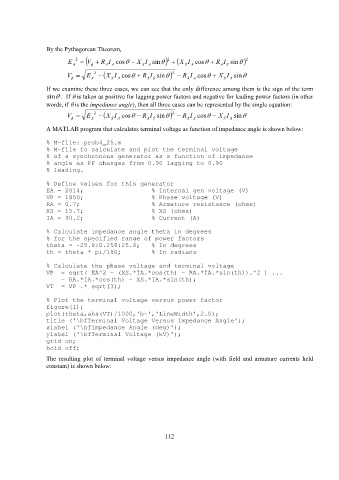
By the Pythagorean Theorem,
2
E A 2    R A I A cos  X S I A sin  V  2  X S I A cos  R A I S sin 

V  E A 2   S I A cos   R A I S sin  X 2  R A I A cos   X S I A sin 

If we examine these three cases, we can see that the only difference among them is the sign of the term
sin  . If  is taken as positive for lagging power factors and negative for leading power factors (in other
words, if  is the impedance angle), then all three cases can be represented by the single equation:
V  E A 2   S I A cos   R A I S sin  X 2  R A I A cos   X S I A sin 


A MATLAB program that calculates terminal voltage as function of impedance angle is shown below:

% M-file: prob4_25.m
% M-file to calculate and plot the terminal voltage
% of a synchronous generator as a function of impedance
% angle as PF changes from 0.90 lagging to 0.90
% leading.

% Define values for this generator
EA = 2814; % Internal gen voltage (V)
VP = 1850; % Phase voltage (V)
RA = 0.7; % Armature resistance (ohms)
XS = 15.7; % XS (ohms)
IA = 90.2; % Current (A)

% Calculate impedance angle theta in degrees
% for the specified range of power factors
theta = -25.8:0.258:25.8; % In degrees
th = theta * pi/180; % In radians

% Calculate the phase voltage and terminal voltage
VP = sqrt( EA^2 - (XS.*IA.*cos(th) - RA.*IA.*sin(th)).^2 ) ...
- RA.*IA.*cos(th) - XS.*IA.*sin(th);
VT = VP .* sqrt(3);

% Plot the terminal voltage versus power factor
figure(1);
plot(theta,abs(VT)/1000,'b-','LineWidth',2.0);
title ('\bfTerminal Voltage Versus Impedance Angle');
xlabel ('\bfImpedance Angle (deg)');
ylabel ('\bfTerminal Voltage (kV)');
grid on;
hold off;
The resulting plot of terminal voltage versus impedance angle (with field and armature currents held
constant) is shown below:

112