Page 137 - Solutions Manual to accompany Electric Machinery Fundamentals

E  V R I  jX I
A  A A S A

 E 1328    0 V  0.3   12.6    0 A  j 2.5  12.6 0 A   1325   1.3 V
A ,nl

 E 1328    0 V  0.3  109 0 A    j 2.5  109 0 A   1324   11.9 V
A ,half


 E 1328 0 V   0.3  209 0 A    j 2.5  209 0 A   1369   22.4 V
A ,full
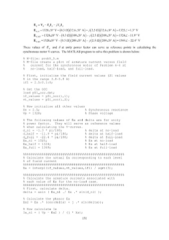
These values of E A and  at unity power factor can serve as reference points in calculating the
synchronous motor V-curves. The MATLAB program to solve this problem is shown below:

% M-file: prob5_5.m
% M-file create a plot of armature current versus field
% current for the synchronous motor of Problem 6-4 at
% no-load, half-load, and full-load.

% First, initialize the field current values (21 values
% in the range 3.8-5.8 A)
if1 = 2.5:0.1:8;

% Get the OCC
load p51_occ.dat;
if_values = p51_occ(:,1);
vt_values = p51_occ(:,2);

% Now initialize all other values
Xs = 2.5; % Synchronous reactance
Vp = 1328; % Phase voltage

% The following values of Ea and delta are for unity
% power factor. They will serve as reference values
% when calculating the V-curves.
d_nl = -1.3 * pi/180; % delta at no-load
d_half = -11.9 * pi/180; % delta at half-load
d_full = -22.4 * pi/180; % delta at full-load
Ea_nl = 1325; % Ea at no-load
Ea_half = 1324; % Ea at half-load
Ea_full = 1369; % Ea at full-load

%%%%%%%%%%%%%%%%%%%%%%%%%%%%%%%%%%%%%%%%%%%%%%%%%%%%%%
% Calculate the actual Ea corresponding to each level
% of field current
%%%%%%%%%%%%%%%%%%%%%%%%%%%%%%%%%%%%%%%%%%%%%%%%%%%%%%
Ea = interp1(if_values,vt_values,if1) / sqrt(3);

%%%%%%%%%%%%%%%%%%%%%%%%%%%%%%%%%%%%%%%%%%%%%%%%%%%%%%
% Calculate the armature currents associated with
% each value of Ea for the no-load case.
%%%%%%%%%%%%%%%%%%%%%%%%%%%%%%%%%%%%%%%%%%%%%%%%%%%%%%
% First, calculate delta.
delta = asin ( Ea_nl ./ Ea .* sin(d_nl) );

% Calculate the phasor Ea
Ea2 = Ea .* (cos(delta) + j .* sin(delta));

% Now calculate Ia
Ia_nl = ( Vp - Ea2 ) / (j * Xs);

131