Page 223 - Intelligent Digital Oil And Gas Fields

Workflow Automation and Intelligent Control 175

The disadvantages of using a VFM based on a physical model are that it can-
not predict unexpected events, memorize previous events, or learn from
previous experience. If changes in pressure, GOR, and water cut are signif-
icant, we suggest using an approach that integrates physical and artificial neu-
ral network (ANN) models. Use the ANN as a VFM in real time, and use the
physical model (updated monthly with test data) to calibrate the ANN.

5.3.5 VFM Based on Artificial Intelligence Models
In KwIDF program (Al-Abbasi et al., 2013), we led a team that designed and
applied a series of automated workflows using AI to provide a VFM model,
with the ultimate goals of filling in missing data, estimating instantaneous
flow rates, and predicting flow rate, WC, and GOR for 7, 15, and 30days
ahead of current production. The work was published in Al-Jasmi et al.
(2013b) and Rebeschini et al. (2013).
These automated workflows are built to predict 30days of production for
gas and ESP artificial lift systems. The workflows use a script to collect the
previous 90days of real-time data (7.7E+6 data points per property) for
these properties: THP; ESP pump frequency; casing head pressure
(CHP); pump discharge pressure (PDP); pump intake pressure (PIP), motor
temperature (MT), and amperage for ESP wells; and CHP, THP, and GL
injection volumes for GL wells. The data are stored in a central data base
and filtered to prepare average daily calculations. The average values are
updated into a well-performance model to train the ANN application sub-
routine. The ANN uses a radial basis function (RBF) algorithm as an acti-
vation function, and the data input in the ANN are saved as text files. The
ANN subroutine checks any changes to detect possible well events, such as
changes in pump frequency or gas injection volume. The output is used to
predict the next day’s liquid rate and WC. The challenge was presented
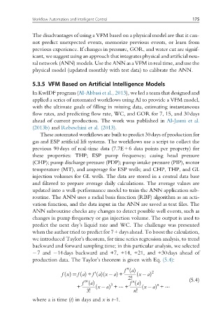
when the author tried to predict for 7+ days ahead. To boost the calculation,
we introduced Taylor’s theorem, for time series regression analysis, to trend
backward and forward sampling time; in this particular analysis, we selected
7 and 14days backward and +7, +14, +21, and +30days ahead of
production data. The Taylor’s theorem is given with Eq. (5.4):

00
a
f ðÞ 2
0
fxðÞ ¼ faðÞ + f aðÞ x að Þ + ð x aÞ
2!
000 n (5.4)
a
f ðÞ 3 f aðÞ n
+ ð x aÞ + ⋯ + ð x aÞ + ⋯
3! n!
where a is time (t) in days and x is t–1.