Page 253 - Intelligent Digital Oil And Gas Fields

Integrated Asset Management and Optimization Workflows 203

30 0
25 –5
20 –10
15 –15
10 –20
5 –25
0 –30
2 2
1 2 1 2
1 1
0 0
0 0
–1 –1 –1 –1
x –2 –2 x –2 –2
2 x 2 x
1 1
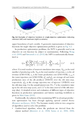
Fig. 6.2 Examples of objective functions in single-objective optimization indicating
minimum (left) and maximum (right) as extrema.
upper boundaries of each variable. A geometric representation of objective
functions for single-objective optimization problem is given in Fig. 6.2.
In production optimization problems, the NPV is generally used as an
objective or cost function Q, subject to maximization. Following Wang
et al. (2009) and Suwartadi et al. (2011) the NPV is mathematically formu-
lated as

" #
N
n
X X r o q r w q n N inj
N prod

o, j w, j X n n
Q ¼ r w, inj q 4t (6.3)
t n inj,l
ð 1+ bÞ
n¼1 j¼1 l¼1
where N is total number of reservoir simulation time-steps, N prod is the total
number of producing wells, N inj is the total number of injectors, r o is the oil
revenue (USD/STB), r w is the water production cost (USD/STB), r w,inj is
n
n
the water injection cost (USD/STB), q o,j and q w,j are average oil and water
production rates of the jth producer (STB/D) over the nth time-step,
n
respectively, q inj,l is the average injection rate of injector l (STB/D) over
n
the nth time-step, b is the annual interest rate (%), t is the cumulative time
n
up to the nth time-step (year), and 4t is the time interval of the nth time-
step (day). A detailed review and evaluation of different types of objective
functions in production optimization and history matching workflows is
given in Mata-Lima (2011).
Traditionally, the solution of the maximizing NPV in oil and gas produc-
tion optimization has been through applying optimal control theory
(Brouwer and Jansen, 2002). The literature mainly refers to two categories
of algorithms used to solve this problem:
• Gradient-based algorithms, where the gradients are derived from the
adjoint method (Brouwer et al., 2004; Sarma et al., 2006, 2008;