Page 269 - Intelligent Digital Oil And Gas Fields

Integrated Asset Management and Optimization Workflows 219

applied to petroleum studies. The reader is encouraged to consider listed ref-
erences for further mathematical detail.

6.3.2 Bayesian Inference and Updating

History matching is a highly nonlinear and ill-posed inverse problem. This
means that depending on the prior information, a set of nonunique solutions
can be obtained that honor both the prior constraints and conditioned data
with associated uncertainty. To assess the uncertainty in estimated reservoir
parameters, one needs to sample the parameters of the posterior distribution.
The Bayesian method provides a very efficient framework to perform this
operation.
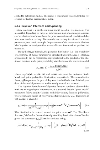
Using the Bayes’ formula, the posterior distribution (i.e., the probability
of occurrence of model parameter m (simulated) given the data d [observed
or measured)] can be represented as proportional to the product of the like-
lihood function and a prior probability distribution of the reservoir model:

p d|m dj mÞp m mðÞ
ð
p m|d mj dð Þ ¼ (6.8)
p d dðÞ
where p mjd (mjd), p dj m (djm), and p m (m) represent the posterior, likeli-
hood, and prior probability distribution, respectively. The normalization
factor p d (d) represents the probability associated with the data. It is indepen-
dent of the model parameters and is usually treated as a constant.
The Bayesian formulation of objective function combines observed data
with the prior geological information. It is assumed that the “prior model”
parameters follow a multi-Gaussian probability density function (pdf ) with a
prior covariance matrix of reservoir model parameters, C M . Therefore, its
pdf, p m (m), is given by

1 1 0 T 1 0

ðÞ
p m m ¼ exp m m C m m (6.9)
M=2 1=2 M
ð 2πÞ j C M j 2
0
This distribution is centered around the prior mean m . The “likelihood
function,” defined as the conditional probability density function of the data
given the parameters p d|m (djm) is calculated using

1 1 T 1
p d|m dj mð Þ ¼ exp ð d gmðÞÞ C ð d gmðÞÞ
N=2 1=2 d
ð 2πÞ j C d j 2
(6.10)