Page 105 - Intermediate Statistics for Dummies

09_045206 ch04.qxd 2/1/07 9:49 AM Page 84
84
Part II: Making Predictions by Using Regression
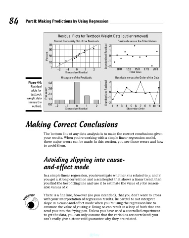
Residual Plots for Textbook Weight Data (outlier removed)
Residuals versus the Fitted Values
99
90
50
10
−2
15.0
20.0
12.5
10.0
17.5
1
2
0
−2
−1
Fitted Value
Standardized Residual
Histogram of the Residuals
Figure 4-6:
Residual
3.6
plots for
2.4
textbook
−1
weight data
1.2
(minus the Frequency Percent 4.8 1 Normal Probability Plot of the Residuals Standardized Residual Standardized Residual −1 2 1 0 2 1 0 Residuals versus the Order of the Data
−2
0.0
outlier). −2 −1 0 1 2 1 2 3 4 5 6 7 8 9 10 11
Standardized Residual Observation Order
Making Correct Conclusions
The bottom line of any data analysis is to make the correct conclusions given
your results. When you’re working with a simple linear regression model,
three major errors can be made. In this section, you see those errors and how
to avoid them.
Avoiding slipping into cause-
and-effect mode
In a simple linear regression, you investigate whether x is related to y, and if
you get a strong correlation and a scatterplot that shows a linear trend, then
you find the best-fitting line and use it to estimate the value of y for reason-
able values of x.
There is a fine line, however (no pun intended), that you don’t want to cross
with your interpretation of regression results. Be careful to not interpret
slope in a cause-and-effect mode when you’re using the regression line to
estimate the value of y using x. Doing so can result in a leap of faith that can
send you into the frying pan. Unless you have used a controlled experiment
to get the data, you can only assume that the variables are correlated; you
can’t really give a stone-cold guarantee why they are related.
@Spy