Page 192 - Intermediate Statistics for Dummies

15_045206 ch09.qxd 2/1/07 10:14 AM Page 171
Chapter 9: Going One-Way with Analysis of Variance
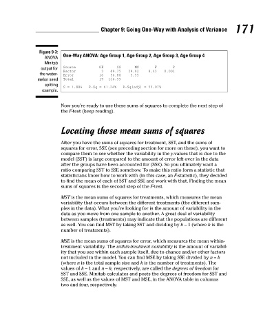
Figure 9-3:
One-Way ANOVA: Age Group 1, Age Group 2, Age Group 3, Age Group 4
ANOVA
Minitab
DF
P
F
Source
SS
MS
output for
8.43
29.92
3
89.75
0.001
Factor
the water-
56.80
16
Error
3.55
Total
melon seed
146.55
19
spitting
S = 1.884 R–Sq = 61.24% R–Sq(adj) = 53.97%
example.
Now you’re ready to use these sums of squares to complete the next step of
the F-test (keep reading).
Locating those mean sums of squares
After you have the sums of squares for treatment, SST, and the sums of 171
squares for error, SSE (see preceding section for more on these), you want to
compare them to see whether the variability in the y-values that is due to the
model (SST) is large compared to the amount of error left over in the data
after the groups have been accounted for (SSE). So you ultimately want a
ratio comparing SST to SSE somehow. To make this ratio form a statistic that
statisticians know how to work with (in this case, an F-statistic), they decided
to find the mean of each of SST and SSE and work with that. Finding the mean
sums of squares is the second step of the F-test.
MST is the mean sums of squares for treatments, which measures the mean
variability that occurs between the different treatments (the different sam-
ples in the data). What you’re looking for is the amount of variability in the
data as you move from one sample to another. A great deal of variability
between samples (treatments) may indicate that the populations are different
as well. You can find MST by taking SST and dividing by k – 1 (where k is the
number of treatments).
MSE is the mean sums of squares for error, which measures the mean within-
treatment variability. The within-treatment variability is the amount of variabil-
ity that you see within each sample itself, due to chance and/or other factors
not included in the model. You can find MSE by taking SSE divided by n – k
(where n is the total sample size and k is the number of treatments). The
values of k – 1 and n – k, respectively, are called the degrees of freedom for
SST and SSE. Minitab calculates and posts the degrees of freedom for SST and
SSE, as well as the values of MST and MSE, in the ANOVA table in columns
two and four, respectively.