Page 194 - Intermediate Statistics for Dummies

15_045206 ch09.qxd 2/1/07 10:14 AM Page 173
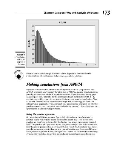
F (3, 16)
0.7
0.6
0.5
0.4
0.3
0.2
Figure 9-4:
F-distribution
0.1
with (3, 16)
degrees of Density 0.8 Chapter 9: Going One-Way with Analysis of Variance 173
0.0
freedom. 1 2 3 4 5 6 7
Be sure to not to exchange the order of the degrees of freedom for the
F-distribution. The difference between F (3, 16) and F (16, 3) is big.
Making conclusions from ANOVA
If you’ve completed the F-test and found your F-statistic (step four in the
ANOVA process), you’re ready for step five of ANOVA: making conclusions for
your hypothesis test of the k population means. If you haven’t already, you
can compare the F-statistic to the corresponding F-distribution with k – 1,
n – k degrees of freedom, to see where it stands and make a conclusion. You
can make the conclusion in one of two ways: the p-value approach or the
critical-value approach. (The approach you use depends primarily on whether
you have access to a computer, especially during exams.) I describe these two
approaches in the following sections.
Using the p-value approach
On Minitab ANOVA output (see Figure 9-3), the value of the F-statistic is
located in the Factor row, under the column noted by F. The associated
p-value for the F-test is located in the Factor row under the column headed
by P. The p-value tells you whether or not you can reject Ho. If the p-value is
less than your prespecified α (typically 0.05), reject Ho. Conclude that the k
population means aren’t all equal and that at least two of them are different.
If the p-value is greater than α, then you can’t reject Ho. You don’t have enough
evidence in your data to say the k population means have any differences.