Page 84 - Intermediate Statistics for Dummies

07_045206 ch03.qxd 2/1/07 9:47 AM Page 63
Chapter 3: Building Confidence and Testing Models
Quantifying power with a power curve
The specific calculations for the power of a hypothesis test are beyond the
scope of this book (so, take that sigh of relief), but computer programs and
graphs are available online to show you what the power is for different hypoth-
esis tests and various sample sizes (just type “power curve for the [blah blah
blah] test” into an Internet search engine). These graphs are called power
curves for a hypothesis test. A power curve is a special kind of graph. It gives
you an idea of how much of a difference from Ho you can detect with the
sample size that you have. Because the precision of your test statistic
increases as your sample size increases, sample size is directly related to
power. But it also depends on how much of a difference from Ho you’re trying
to detect. For example, if a package delivery company claims that its pack-
ages arrive in 2 days or less, do you want to blow the whistle if it’s actually
2.1 days? Or wait until it’s 3 days? You need a much larger sample size to
detect the 2.1-days situation versus the 3-days situation just because of the
precision level needed.
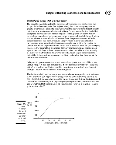
In Figure 3-1, you can see the power curve for a particular test of Ho: µ = 0 63
versus Ha: µ > 0. You can assume that σ (the standard deviation of the popu-
lation) is equal to two (I give you this value in each problem) and doesn’t
change. I set the sample size at ten throughout.
The horizontal (x) axis on the power curve shows a range of actual values of
µ. For example, you hypothesize that µ is equal to 0, but it may actually be
0.5, 1.0, 2.0, 3.0, or any other possible value. If µ equals 0, then Ho is true, and
the chance of detecting this (rejecting Ho) is equal to 0.05, the set value of α.
You work from that baseline. So, on the graph in Figure 3-1, when x = 0, you
get a y-value of 0.05.
1.0
0.8
Power
Figure 3-1:
(n=10)
Power 0.6
curve for
Ho: µ = 0 0.4
versus Ha:
0.2
µ > 0, for
n = 10 and
σ = 2. 0.5 1.0 1.5 2.0 2.5 3.0
Actual Value of the Parameter