Page 85 - Intermediate Statistics for Dummies

07_045206 ch03.qxd 2/1/07 9:47 AM Page 64
64
Part I: Data Analysis and Model-Building Basics
Suppose that µ is actually 0.5, not 0, as you hypothesized. A computer tells
you that the chance of rejecting Ho (what you’re supposed to do here) is
0.197 = 0.20, which is the power. So, you have about a 20 percent chance of
detecting this difference with a sample size of ten. As you move to the right,
away from zero on the horizontal (x) axis, you can see that the power goes
up, and the y-values get closer and closer to 1.0.
For example, if the actual value of µ is 1.0, the difference from 0 is easier to
detect than if it’s 0.50. In fact, the power at 1.0 is equal to 0.475 = 0.48, so you
have almost a 50 percent chance of catching the difference from Ho in this
case. And as the values of the mean increase, the power gets closer and
closer to 1.0. Power never reaches 1.0, because statistics can never prove
anything with 100 percent accuracy. But you can get close to 1.0 if the actual
value is far enough from your hypothesis.
Controlling the sample size
You don’t have any control over what the actual value of the parameter is,
though, because that number is unknown. So what do you have control over?
The sample size. As the sample size increases, it becomes easier to detect a
real difference from Ho.
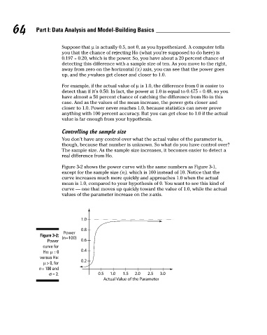
Figure 3-2 shows the power curve with the same numbers as Figure 3-1,
except for the sample size (n), which is 100 instead of 10. Notice that the
curve increases much more quickly and approaches 1.0 when the actual
mean is 1.0, compared to your hypothesis of 0. You want to see this kind of
curve — one that moves up quickly toward the value of 1.0, while the actual
values of the parameter increase on the x-axis.
1.0
0.8
Power
Figure 3-2: (n=100)
Power 0.6
curve for
Ho: µ = 0 0.4
versus Ha:
µ > 0, for 0.2
n = 100 and
σ = 2. 0.5 1.0 1.5 2.0 2.5 3.0
Actual Value of the Parameter