Page 86 - Intermediate Statistics for Dummies

07_045206 ch03.qxd 2/1/07 9:47 AM Page 65
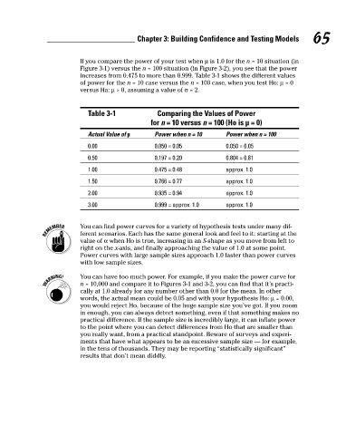
If you compare the power of your test when µ is 1.0 for the n = 10 situation (in
Figure 3-1) versus the n = 100 situation (in Figure 3-2), you see that the power
increases from 0.475 to more than 0.999. Table 3-1 shows the different values
of power for the n = 10 case versus the n = 100 case, when you test Ho: µ = 0
versus Ha: µ > 0, assuming a value of σ = 2.
Comparing the Values of Power
Table 3-1
for n = 10 versus n = 100 (Ho is µ = 0)
Power when n = 10
Actual Value of µ
Power when n = 100
0.050 = 0.05
0.00
0.050 = 0.05
0.197 = 0.20
0.50
0.804 = 0.81
approx. 1.0
0.475 = 0.48
1.00
0.766 = 0.77
1.50
approx. 1.0
2.00 Chapter 3: Building Confidence and Testing Models 65
0.935 = 0.94
approx. 1.0
3.00 0.999 = approx. 1.0 approx. 1.0
You can find power curves for a variety of hypothesis tests under many dif-
ferent scenarios. Each has the same general look and feel to it: starting at the
value of α when Ho is true, increasing in an S-shape as you move from left to
right on the x-axis, and finally approaching the value of 1.0 at some point.
Power curves with large sample sizes approach 1.0 faster than power curves
with low sample sizes.
You can have too much power. For example, if you make the power curve for
n = 10,000 and compare it to Figures 3-1 and 3-2, you can find that it’s practi-
cally at 1.0 already for any number other than 0.0 for the mean. In other
words, the actual mean could be 0.05 and with your hypothesis Ho: µ = 0.00,
you would reject Ho, because of the huge sample size you’ve got. If you zoom
in enough, you can always detect something, even if that something makes no
practical difference. If the sample size is incredibly large, it can inflate power
to the point where you can detect differences from Ho that are smaller than
you really want, from a practical standpoint. Beware of surveys and experi-
ments that have what appears to be an excessive sample size — for example,
in the tens of thousands. They may be reporting “statistically significant”
results that don’t mean diddly.