Page 334 - Intro to Tensor Calculus

328

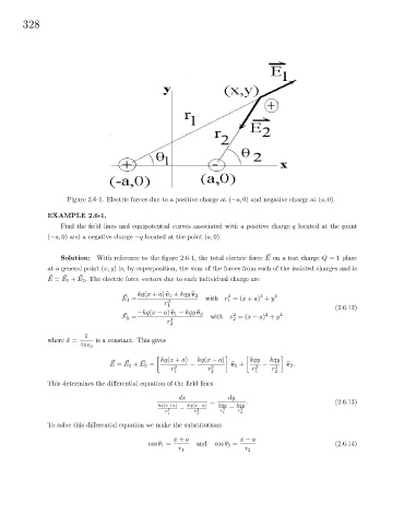
Figure 2.6-1. Electric forces due to a positive charge at (−a, 0) and negative charge at (a, 0).

EXAMPLE 2.6-1.
Find the field lines and equipotential curves associated with a positive charge q located at the point
(−a, 0) and a negative charge −q located at the point (a, 0).

~
Solution: With reference to the figure 2.6-1, the total electric force E on a test charge Q = 1 place
at a general point (x, y) is, by superposition, the sum of the forces from each of the isolated charges and is
~
~
~
E = E 1 + E 2 . The electric force vectors due to each individual charge are
2
2
~
E 1 = kq(x + a) b e 1 + kqy b e 2 with r =(x + a) + y 2
1
r 3 1
(2.6.12)
~
2
2
E 2 = −kq(x − a) b e 1 − kqy b e 2 with r =(x − a) + y 2
2
3
r 2
1
where k = is a constant. This gives
4π 0

kq(x + a) kq(x − a) kqy kqy
~
~
~
E = E 1 + E 2 = − b e 1 + − b e 2 .
r 1 3 r 3 2 r 3 1 r 3 2
This determines the differential equation of the field lines
dx dy
= . (2.6.13)
kq(x+a) kq(x−a) kqy kqy
r 3 − r 3 r 3 − r 3
1 2 1 2
To solve this differential equation we make the substitutions
x + a x − a
cos θ 1 = and cos θ 2 = (2.6.14)
r 1 r 2