Page 335 - Intro to Tensor Calculus

329

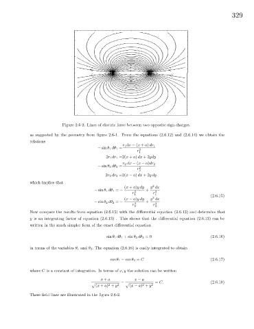
Figure 2.6-2. Lines of electric force between two opposite sign charges.

as suggested by the geometry from figure 2.6-1. From the equations (2.6.12) and (2.6.14) we obtain the
relations
r 1 dx − (x + a) dr 1
− sin θ 1 dθ 1 = 2
r 1
2r 1 dr 1 =2(x + a) dx +2ydy
r 2 dx − (x − a)dr 2
− sin θ 2 dθ 2 =
r 2
2
2r 2 dr 2 =2(x − a) dx +2ydy
which implies that
2
(x + a)ydy y dx
− sin θ 1 dθ 1 = − 3 + 3
r r
1 1 (2.6.15)
2
(x − a)ydy y dx
− sin θ 2 dθ 2 = − 3 + 3
r r
2 2
Now compare the results from equation (2.6.15) with the differential equation (2.6.13) and determine that
y is an integrating factor of equation (2.6.13) . This shows that the differential equation (2.6.13) can be
written in the much simpler form of the exact differential equation

− sin θ 1 dθ 1 +sin θ 2 dθ 2 =0 (2.6.16)

in terms of the variables θ 1 and θ 2 . The equation (2.6.16) is easily integrated to obtain

cos θ 1 − cos θ 2 = C (2.6.17)

where C is a constant of integration. In terms of x, y the solution can be written

x + a x − a
p − p = C. (2.6.18)
2
2
(x + a) + y 2 (x − a) + y 2
These field lines are illustrated in the figure 2.6-2.