Page 94 - Intro to Tensor Calculus

89

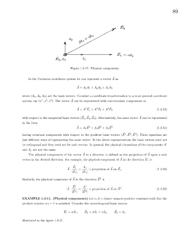
Figure 1.3-17. Physical components

~
In the Cartesian coordinate system we can represent a vector A as
~
A = A x b e 1 + A y b e 2 + A z b e 3

where ( b e 1 , b e 2 , b e 3 ) are the basis vectors. Consider a coordinate transformation to a more general coordinate
2
1
~
3
system, say (x ,x ,x ). The vector A can be represented with contravariant components as
~ 1 ~ 2 ~ 3 ~
A = A E 1 + A E 2 + A E 3 (1.3.53)
~
~
~
~
with respect to the tangential basis vectors (E 1 , E 2 , E 3 ). Alternatively, the same vector A can be represented
in the form
~ 1
~ 3
~
~ 2
A = A 1 E + A 2 E + A 3 E (1.3.54)
~ 1 ~ 2 ~ 3
having covariant components with respect to the gradient basis vectors (E , E , E ). These equations are
just different ways of representing the same vector. In the above representations the basis vectors need not
be orthogonal and they need not be unit vectors. In general, the physical dimensions of the components A i
and A j are not the same.
~
~
The physical components of the vector A in a direction is defined as the projection of A upon a unit
~
~
vector in the desired direction. For example, the physical component of A in the direction E 1 is
~
~ E 1 A 1 ~ ~
A · = = projection of A on E 1 . (1.3.58)
~
~
|E 1 | |E 1 |
~
~ 1
Similarly, the physical component of A in the direction E is
~ 1
E A 1
~ ~ ~ 1
A · = = projection of A on E . (1.3.59)
~ 1 ~ 1
|E | |E |
EXAMPLE 1.3-11. (Physical components) Let α, β, γ denote nonzero positive constants such that the
product relation αγ = 1 is satisfied. Consider the nonorthogonal basis vectors
~
~
~
E 1 = α b e 1 , E 2 = β b e 1 + γ b e 2 , E 3 = b e 3
illustrated in the figure 1.3-17.