Page 90 - Intro to Tensor Calculus

85

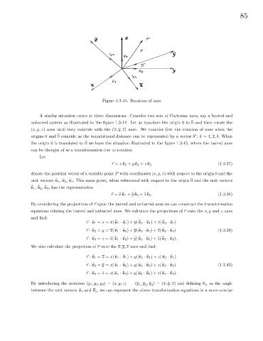
Figure 1.3-15. Rotation of axes

A similar situation exists in three dimensions. Consider two sets of Cartesian axes, say a barred and
unbarred system as illustrated in the figure 1.3-14. Let us translate the origin 0 to 0 and then rotate the
(x, y, z) axes until they coincide with the (x, y, z) axes. We consider first the rotation of axes when the
k
origins 0 and 0 coincide as the translational distance can be represented by a vector b ,k =1, 2, 3. When
the origin 0 is translated to 0 we have the situation illustrated in the figure 1.3-15, where the barred axes
can be thought of as a transformation due to rotation.
Let
r (1.3.37)
~ = x b e 1 + y b e 2 + z b e 3
denote the position vector of a variable point P with coordinates (x, y, z) with respect to the origin 0 and the
unit vectors b e 1 , b e 2 , b e 3 . This same point, when referenced with respect to the origin 0 and the unit vectors
ˆ ˆ ˆ
e 1 , e 2 , e 3 , has the representation
r ˆ ˆ ˆ (1.3.38)
~ = x e 1 + y e 2 + z e 3 .
By considering the projections of ~ upon the barred and unbarred axes we can construct the transformation
r
equations relating the barred and unbarred axes. We calculate the projections of ~ onto the x, y and z axes
r
and find:
~ · b e 1 = x = x( e 1 · b e 1 )+ y( e 2 · b e 1 )+ z( e 3 · b e 1 )
r ˆ ˆ ˆ
~ · b e 2 = y = x( e 1 · b e 2 )+ y( e 2 · b e 2 )+ z( e 3 · b e 2 )
r ˆ ˆ ˆ (1.3.39)
~ · b e 3 = z = x( e 1 · b e 3 )+ y( e 2 · b e 3 )+ z( e 3 · b e 3 ).
r ˆ ˆ ˆ
r
We also calculate the projection of ~ onto the x, y, z axes and find:
~ · e 1 = x = x( b e 1 · e 1 )+ y( b e 2 · e 1 )+ z( b e 3 · e 1 )
r ˆ ˆ ˆ ˆ
~ · e 2 = y = x( b e 1 · e 2 )+ y( b e 2 · e 2 )+ z( b e 3 · e 2 )
r ˆ ˆ ˆ ˆ (1.3.40)
~ · e 3 = z = x( b e 1 · e 3 )+ y( b e 2 · e 3 )+ z( b e 3 · e 3 ).
r ˆ ˆ ˆ ˆ
By introducing the notation (y 1 ,y 2 ,y 3 )= (x, y, z) (y , y , y )=(x, y, z) and defining θ ij as the angle
3
1
2
ˆ
between the unit vectors b e i and e j , we can represent the above transformation equations in a more concise