Page 93 - Intro to Tensor Calculus

88

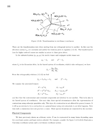
Figure 1.3-16. Transformation to curvilinear coordinates

These are the transformation laws when moving from one orthogonal system to another. In this case the
direction cosines ` im are constants and satisfy the relations given in equation (1.3.45). The transformation
laws for higher ordered tensors are similar in nature to those given above.
In the unbarred system (y 1 ,y 2 ,y 3) the metric tensor and conjugate metric tensor are:

and g ij
g ij = δ ij = δ ij
where δ ij is the Kronecker delta. In the barred system of coordinates, which is also orthogonal, we have

∂y m ∂y m
g = .
ij
∂y ∂y
i j
From the orthogonality relations (1.3.45) we find

g ij = ` mi ` mj = δ ij and g ij = δ ij .

We examine the associated tensors
i ij j
A = g A j A i = g ij A
ij
A = g im jn A mn = g mi g nj A ij
g A mn
i
i
A = g im A mn A = g nj A ij
n
n
and find that the contravariant and covariant components are identical to one another. This holds also in
the barred system of coordinates. Also note that these special circumstances allow the representation of
contractions using subscript quantities only. This type of a contraction is not allowed for general tensors. It
is left as an exercise to try a contraction on a general tensor using only subscripts to see what happens. Note
that such a contraction does not produce a tensor. These special situations are considered in the exercises.

Physical Components

~
We have previously shown an arbitrary vector A can be represented in many forms depending upon
the coordinate system and basis vectors selected. For example, consider the figure 1.3-16 which illustrates a
Cartesian coordinate system and a curvilinear coordinate system.