Page 106 -

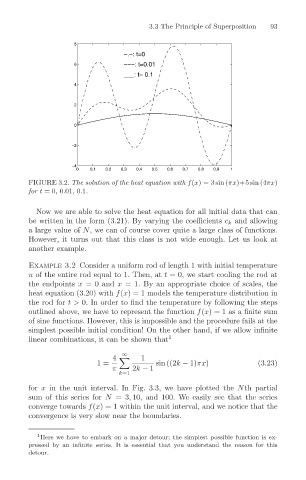
−−−: t=0.01
___: t= 0.1
−2 8 6 4 2 0 −.−: t=0 3.3 The Principle of Superposition 93
−4
0 0.1 0.2 0.3 0.4 0.5 0.6 0.7 0.8 0.9 1
FIGURE 3.2. The solution of the heat equation with f(x) = 3 sin (πx)+5 sin (4πx)
for t =0, 0.01, 0.1.

Now we are able to solve the heat equation for all initial data that can
be written in the form (3.21). By varying the coefficients c k and allowing
a large value of N, we can of course cover quite a large class of functions.
However, it turns out that this class is not wide enough. Let us look at
another example.

Example 3.2 Consider a uniform rod of length 1 with initial temperature
u of the entire rod equal to 1. Then, at t = 0, we start cooling the rod at
the endpoints x = 0 and x = 1. By an appropriate choice of scales, the
heat equation (3.20) with f(x) = 1 models the temperature distribution in
the rod for t> 0. In order to find the temperature by following the steps
outlined above, we have to represent the function f(x) = 1 as a finite sum
of sine functions. However, this is impossible and the procedure fails at the
simplest possible initial condition! On the other hand, if we allow infinite
linear combinations, it can be shown that 1

∞
4 1
1= sin ((2k − 1)πx) (3.23)
π 2k − 1
k=1
for x in the unit interval. In Fig. 3.3, we have plotted the Nth partial
sum of this series for N =3, 10, and 100. We easily see that the series
converge towards f(x) = 1 within the unit interval, and we notice that the
convergence is very slow near the boundaries.

1 Here we have to embark on a major detour; the simplest possible function is ex-
pressed by an infinite series. It is essential that you understand the reason for this
detour.