Page 108 -

0.8
−−−: t=0.01
___: t= 0.1
0.6
0.4
0.2 1 −.−: t=0 3.4 Fourier Coefficients 95
0
0 0.1 0.2 0.3 0.4 0.5 0.6 0.7 0.8 0.9 1
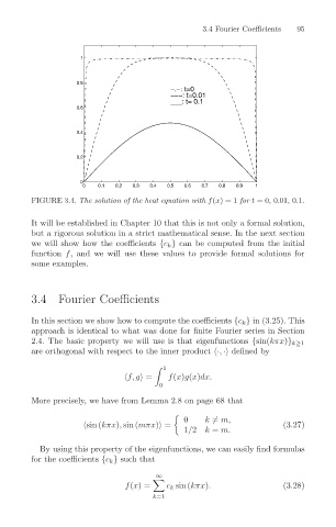
FIGURE 3.4. The solution of the heat equation with f(x)=1 for t =0, 0.01, 0.1.
It will be established in Chapter 10 that this is not only a formal solution,
but a rigorous solution in a strict mathematical sense. In the next section
we will show how the coefficients {c k } can be computed from the initial
function f, and we will use these values to provide formal solutions for
some examples.

3.4 Fourier Coefficients

In this section we show how to compute the coefficients {c k } in (3.25). This
approach is identical to what was done for finite Fourier series in Section
2.4. The basic property we will use is that eigenfunctions {sin(kπx)} k≥1
are orthogonal with respect to the inner product
·, ·( defined by

1

f, g = f(x)g(x)dx.
0
More precisely, we have from Lemma 2.8 on page 68 that

0 k = m,

sin (kπx), sin (mπx) = (3.27)
1/2 k = m.
By using this property of the eigenfunctions, we can easily find formulas
for the coefficients {c k } such that
∞

f(x)= c k sin (kπx). (3.28)
k=1