Page 155 -

4. Finite Difference Schemes For The Heat Equation
142

m

j+1
j
j-1 m+1
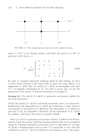
FIGURE 4.7. The computational molecule of the implicit scheme.
where I ∈ R n,n is the identity matrix, and where the matrix A ∈ R n,n is
given by (4.16) above, i.e.
 
2 −1 0 ... 0
. .
 . . 
−1 2 −1 . .
 
1  . . . 
A =  0 . . . . . . 0  . (4.40)


2
(∆x)  
.
. .
 . 
 . . −1 2 −1 
0 ... 0 −1 2
In order to compute numerical solutions based on this scheme, we have
to solve linear systems of the form (4.39) at each time step. Hence, it is
important to verify that the matrix (I +∆tA) is nonsingular such that
m
v m+1 is uniquely determined by v . In order to prove this, we use the
properties of the matrix A derived in Lemma 2.9 on page 70.
Lemma 4.1 The matrix (I +∆tA) is symmetric and positive definite for
all mesh parameters.
Proof: The matrix (I +∆tA) is obviously symmetric, since A is symmetric.
Furthermore, the eigenvalues of (I +∆tA) are of the form 1+∆tµ, where µ
corresponds to eigenvalues of A. However, the eigenvalues of A, which are
given by (4.12), are all positive. Therefore, all the eigenvalues of (I +∆tA)
are positive, and hence this matrix is positive definite.

Since (I +∆tA) is symmetric and positive definite, it follows from Propo-
sition 2.4 that the system (4.39) has a unique solution that can be computed
using the Gaussian elimination procedure given in Algorithm 2.1 on page
53. From a computational point of view, it is important to note that the
coefficient matrix (I +∆tA) in (4.39) does not change in time. This obser-