Page 156 -

4.4 An Implicit Scheme
0.35
0.3
0.25
0.2
0.15
0.1
0.05 dx=0.02, dt=0.000201, r=0.5025 143
0
0 0.1 0.2 0.3 0.4 0.5 0.6 0.7 0.8 0.9 1
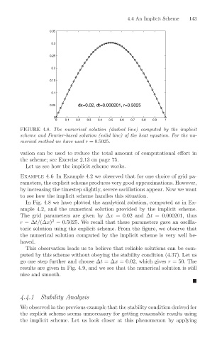
FIGURE 4.8. The numerical solution (dashed line) computed by the implicit
scheme and Fourier-based solution (solid line) of the heat equation. For the nu-
merical method we have used r =0.5025.
vation can be used to reduce the total amount of computational effort in
the scheme; see Exercise 2.13 on page 75.
Let us see how the implicit scheme works.
Example 4.6 In Example 4.2 we observed that for one choice of grid pa-
rameters, the explicit scheme produces very good approximations. However,
by increasing the timestep slightly, severe oscillations appear. Now we want
to see how the implicit scheme handles this situation.
In Fig. 4.8 we have plotted the analytical solution, computed as in Ex-
ample 4.2, and the numerical solution provided by the implicit scheme.
The grid parameters are given by ∆x =0.02 and ∆t =0.000201, thus
r =∆t/(∆x) =0.5025. We recall that these parameters gave an oscilla-
2
toric solution using the explicit scheme. From the figure, we observe that
the numerical solution computed by the implicit scheme is very well be-
haved.
This observation leads us to believe that reliable solutions can be com-
puted by this scheme without obeying the stability condition (4.37). Let us
go one step further and choose ∆t =∆x =0.02, which gives r = 50. The
results are given in Fig. 4.9, and we see that the numerical solution is still
nice and smooth.

4.4.1 Stability Analysis
We observed in the previous example that the stability condition derived for
the explicit scheme seems unnecessary for getting reasonable results using
the implicit scheme. Let us look closer at this phenomenon by applying