Page 63 -

2. Two-Point Boundary Value Problems
50
h
n
Rate of convergence
E h
5
0.0058853
1/6
1.969
0.0017847
1/11
10
1/21
1.996
0.0004910
20
40
1/41
2.000
0.0001288
2.000
1/81
80
0.0000330
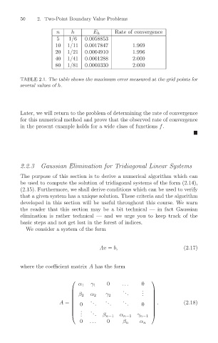
TABLE 2.1. The table shows the maximum error measured at the grid points for
several values of h.
Later, we will return to the problem of determining the rate of convergence
for this numerical method and prove that the observed rate of convergence
in the present example holds for a wide class of functions f.

2.2.3 Gaussian Elimination for Tridiagonal Linear Systems
The purpose of this section is to derive a numerical algorithm which can
be used to compute the solution of tridiagonal systems of the form (2.14),
(2.15). Furthermore, we shall derive conditions which can be used to verify
that a given system has a unique solution. These criteria and the algorithm
developed in this section will be useful throughout this course. We warn
the reader that this section may be a bit technical — in fact Gaussian
elimination is rather technical — and we urge you to keep track of the
basic steps and not get lost in the forest of indices.
We consider a system of the form
Av = b, (2.17)
where the coefficient matrix A has the form
 
0 ... 0
γ 1
α 1
. .
 . . 
 β 2 α 2 γ 2 . . 
 
. . .
 . . . 
A =  0 . . . 0  . (2.18)
 
 . .
 . . . . β n−1 α n−1 γ n−1 

0 ... 0 β n α n