Page 66 -

2.2 A Finite Difference Approximation
53
However, from this bidiagonal system we can easily compute the solution
v. From the last equation, we have
c n
v n =
,
(2.24)
δ n
and by tracking the system backwards we find
,
v k =
k = n − 1,n − 2,... , 1 .
(2.25)
c k − γ k v k+1
δ k
Hence, we have derived an algorithm for computing the solution v of the
original tridiagonal system (2.19). First we compute the variables δ j and
c j from the relations (2.22) with k = n, and then we compute the solution
v from (2.24) and (2.25).
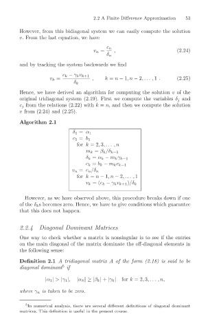
Algorithm 2.1
δ 1 = α 1
c 1 = b 1
for k =2, 3,... ,n
m k = β k /δ k−1
δ k = α k − m k γ k−1
c k = b k − m k c k−1
v n = c n /δ n
for k = n − 1,n − 2,... , 1
v k =(c k − γ k v k+1 )/δ k
However, as we have observed above, this procedure breaks down if one
of the δ k s becomes zero. Hence, we have to give conditions which guarantee
that this does not happen.
2.2.4 Diagonal Dominant Matrices
One way to check whether a matrix is nonsingular is to see if the entries
on the main diagonal of the matrix dominate the off-diagonal elements in
the following sense:
Definition 2.1 A tridiagonal matrix A of the form (2.18) is said to be
diagonal dominant if
5
|α 1 | > |γ 1 |, |α k |≥|β k | + |γ k | for k =2, 3,... ,n,
where γ n is taken to be zero.

5 In numerical analysis, there are several different definitions of diagonal dominant
matrices. This definition is useful in the present course.