Page 64 -

51
2.2 A Finite Difference Approximation
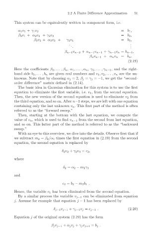
This system can be equivalently written in component form, i.e.
= b 1 ,
α 1 v 1 + γ 1 v 2
= b 2 ,
β 2 v 1 + α 2 v 2 + γ 2 v 3
= b 3 ,
β 3 v 2 + α 3 v 3 +
γ 3 v 4
.
.
.
.
.
.
β n−1 v n−2 + α n−1 v n−1 + γ n−1 v n = b n−1 ,
β n v n−1 + α n v n = b n .
(2.19)
Here the coefficients β 2 ,... ,β n , α 1 ,... ,α n , γ 1 ,... ,γ n−1 , and the right-
hand side b 1 ,... ,b n are given real numbers and v 1 ,v 2 ,... ,v n are the un-
knowns. Note that by choosing α j =2,β j = γ j = −1, we get the “second-
order difference” matrix defined in (2.14).
The basic idea in Gaussian elimination for this system is to use the first
equation to eliminate the first variable, i.e. v 1 , from the second equation.
Then, the new version of the second equation is used to eliminate v 2 from
the third equation, and so on. After n−1 steps, we are left with one equation
containing only the last unknown v n . This first part of the method is often
referred to as the “forward sweep.”
Then, starting at the bottom with the last equation, we compute the
value of v n , which is used to find v n−1 from the second from last equation,
and so on. This latter part of the method is referred to as the “backward
sweep.”
With an eye to this overview, we dive into the details. Observe first that if
we subtract m 2 = β 2 /α 1 times the first equation in (2.19) from the second
equation, the second equation is replaced by
δ 2 v 2 + γ 2 v 3 = c 2 ,
where
and δ 2 = α 2 − m 2 γ 1
c 2 = b 2 − m 2 b 1 .
Hence, the variable v 1 has been eliminated from the second equation.
By a similar process the variable v j−1 can be eliminated from equation
j. Assume for example that equation j − 1 has been replaced by

δ j−1 v j−1 + γ j−1 v j = c j−1 . (2.20)
Equation j of the original system (2.19) has the form

β j v j−1 + α j v j + γ j v j+1 = b j .