Page 357 - Introduction to AI Robotics

340
H20 H8 H9 H10 9 Topological Path Planning
H11
R7
H12
R4
H7 R5 H13
R6
H1
H2 H3 H4 H5 H6 F1 H14 H15

R1 R2 R3

H19 H18 F2 H17 H16

a.

R7 H20 H8 H9 H10 H11 R7* H20 H8 Hd9 H10 H11

H1 R6 H7 R5 H13 R4 H12 Hd1 Hd7 R5 Hd13 R4 Hd12
H2 H3 H4 H5 H6 F1 H14 H15 H2 H3 H4 Hd5 H6 F1 H14 H15
R1 R2 R3 R2 R3*

H19 H18 F2 H17 H16 H19 Hd18 F2 Hd17 H16
b. c.

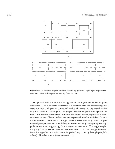
Figure 9.11 a.) Metric map of an office layout, b.) graphical topological representa-
tion, and c.) refined graph for traveling from R3 to R7.

An optimal path is computed using Dijkstra’s single source shortest path
algorithm. The algorithm generates the shortest path by considering the
costs between each pair of connected nodes; the costs are expressed as the
length or weight of an edge in the graph. Since the topological representa-
tion is not metric, connections between the nodes reflect preferences in con-
structing routes. These preferences are expressed as edge weights. In this
implementation, navigating through foyers was considerably more compu-
tationally expensive and unreliable; therefore the edge weighting for any
path subsegment originating from a foyer was set at 3. The edge weight
for going from a room to another room was set at 2 to discourage the robot
from finding solutions which were “impolite” (e.g., cutting through people’s
offices). All other connections were set to 1.