Page 379 - Introduction to AI Robotics

362

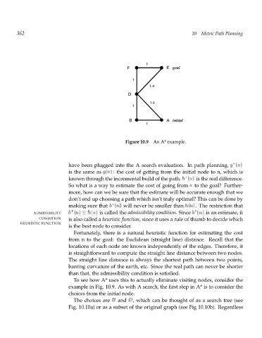
Figure 10.9 An A* example. 10 Metric Path Planning

have been plugged into the A search evaluation. In path planning, g (n)
is thesameas g(n): the cost of getting from the initial node to n, which is

known through the incremental build of the path. h (n) is the real difference.
So what is a way to estimate the cost of going from n to the goal? Further-
more, how can we be sure that the estimate will be accurate enough that we
don’t end up choosing a path which isn’t truly optimal? This can be done by

making sure that h (n) will never be smaller than h(n). The restriction that

ADMISSIBILITY h (n) h(n) is called the admissibility condition.Since h (n) is an estimate, it
CONDITION is also called a heuristic function, since it uses a rule of thumb to decide which
HEURISTIC FUNCTION
is the best node to consider.
Fortunately, there is a natural heuristic function for estimating the cost
from n to the goal: the Euclidean (straight line) distance. Recall that the
locations of each node are known independently of the edges. Therefore, it
is straightforward to compute the straight line distance between two nodes.
The straight line distance is always the shortest path between two points,
barring curvature of the earth, etc. Since the real path can never be shorter
than that, the admissibility condition is satisfied.
To see how A* uses this to actually eliminate visiting nodes, consider the
example in Fig. 10.9. As with A search, the first step in A* is to consider the
choices from the initial node.
The choices are B and D, which can be thought of as a search tree (see
Fig. 10.10a) or as a subset of the original graph (see Fig 10.10b). Regardless