Page 428 - Introduction to AI Robotics

11.6 Comparison of Methods
(0 :14)(0 :5) 411
m(dontknow ) = = :12 0
1:0 (0 :86)(0 :5)
(0 :14)(0 :5)
mpty
m(E ) = = :12 0
1:0 (0 :86)(0 :5)
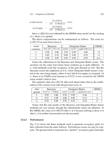
Since g r[3][10] i d is not affected by the HIMM sonar model for the reading
at t 3 , there is no update.
The above computations can be summarized as follows. The score for
g r[3][10] i d at each observation is:
sonar Bayesian Dempster-Shafer HIMM
certainty: P (sjO) P (sjE) m(O) m(E) m(dontknow )
t 1 0.54 0.46 0.56 0.00 0.46 +3
t 2 0.69 0.31 0.69 0.00 0.31 +3
t 3 0.50 0.50 0.00 0.50 0.50 n/a
Notice the differences in the Bayesian and Dempster-Shafer scores. The
numbers are the same, but where those numbers go is quite different. At
t 2 , both methods score the occupancy of the grid element as 0.69. But the
Bayesian scores the emptiness as 0.31, while Dempster-Shafer doesn’t com-
mit to the area being empty; rather it can’t tell if it is empty or occupied. At
t 3 , there is no HIMM score because g r[3][10] i d is not covered by the HIMM
sonar model’s field of view.
The updated value of g r[3][10] i d after each observation, that is, the combi-
nation of the current score with the previous score, is:
after Bayesian Dempster-Shafer HIMM
update: P (Ojs) P (Ejs) m(O) m(E) m(dontknow )
t 1 0.54 0.46 0.54 0.00 0.46 3
t 2 0.72 0.28 0.86 0.00 0.14 6
t 3 0.72 0.28 0.76 0.12 0.12 6
Notice that the end results of the Bayesian and Dempster-Shafer fusion
methods are very similar, though the intermediate values are different. In
the HIMM, the value of g r[3][10] i d after t 3 is 6 because nothing is done to it
after t 2 ; it is neither incremented nor decremented.

11.6.2 Performance
Fig. 11.14 shows the three methods used to generate occupancy grids for
data collected from the same hallway. Performance scores are easy to com-
pute. The ground truth is expressed as a “perfect” occupancy grid, manually