Page 423 - Introduction to AI Robotics

406
Localization and Map Making
11
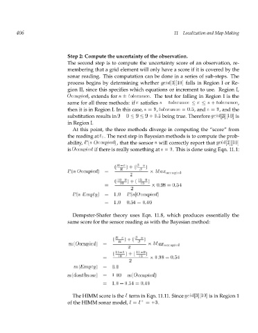
Step 2: Compute the uncertainty of the observation.
The second step is to compute the uncertainty score of an observation, re-
membering that a grid element will only have a score if it is covered by the
sonar reading. This computation can be done in a series of sub-steps. The
process begins by determining whether g r[3][10] i d falls in Region I or Re-
gion II, since this specifies which equations or increment to use. Region I,
,
exten
O c c u p i e dds for s tolerance . The test for falling in Region I is the
nce
same for all three methods: if r satisfies s tolerance r s + tolera ,
then it is in Region I. In this case, s = , tolerance = :5,and r = ,and the 9 0 9
substitution results in 9 0 9 9 :5 being true. Th +erefore g r[3][10] i d is 0
in Region I.
At this point, the three methods diverge in computing the “score” from
the reading at t 1 . The next step in Bayesian methods is to compute the prob-
t
,
)
ha
t
ability, P (sjO c c u p i e dhe sensor s will correctly report that g r[3][10] i d
t
is O if there is really something at s = . This is done using Eqn. 11.1: 9
ccupied
( R R r ) ) + (
P (sjO ) = M occupied a x
ccupied
2
( 10 9 ) 15 0 ) + (
= 10 15 0:9 :54 8 = 0
2
P (sjE ) m= 1:0 p P (sjO y )
ccupied
t
= 1:0 0:54= :46
0
Dempster-Shafer theory uses Eqn. 11.8, which produces essentially the
same score for the sensor reading as with the Bayesian method:
( R R r ) ) + (
ccupied
m(O ) = M occupied a x
2
( 10 9 ) 15 0 ) + (
= 10 15 0:98=0 :54
2
m(E ) m= 0:0 p t y
m(dontknow ) = 1:00 m(O )
ccupied
= 1:0 0:5 :46 4 = 0

The HIMM score is the I term in Eqn. 11.11. Since g r[3][10] i d is in Region 1
of the HIMM sonar model, I = I + = . + 3