Page 434 - Introduction to AI Robotics

417
11.7 Localization
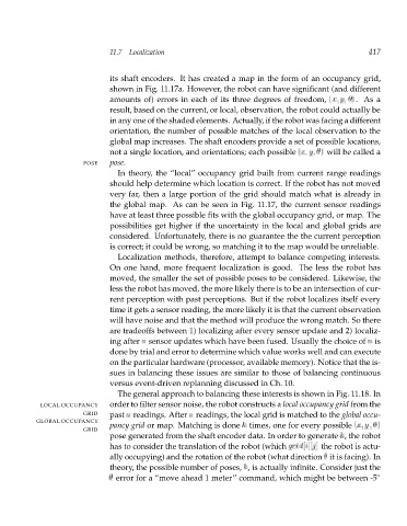
its shaft encoders. It has created a map in the form of an occupancy grid,
shown in Fig. 11.17a. However, the robot can have significant (and different
amounts of) errors in each of its three degrees of freedom, (x;y; ).As a
result, based on the current, or local, observation, the robot could actually be
in any one of the shaded elements. Actually, if the robot was facing a different
orientation, the number of possible matches of the local observation to the
global map increases. The shaft encoders provide a set of possible locations,
not a single location, and orientations; each possible (x;y; ) will be called a
POSE pose.
In theory, the “local” occupancy grid built from current range readings
should help determine which location is correct. If the robot has not moved
very far, then a large portion of the grid should match what is already in
the global map. As can be seen in Fig. 11.17, the current sensor readings
have at least three possible fits with the global occupancy grid, or map. The
possibilities get higher if the uncertainty in the local and global grids are
considered. Unfortunately, there is no guarantee the the current perception
is correct; it could be wrong, so matching it to the map would be unreliable.
Localization methods, therefore, attempt to balance competing interests.
On one hand, more frequent localization is good. The less the robot has
moved, the smaller the set of possible poses to be considered. Likewise, the
less the robot has moved, the more likely there is to be an intersection of cur-
rent perception with past perceptions. But if the robot localizes itself every
time it gets a sensor reading, the more likely it is that the current observation
will have noise and that the method will produce the wrong match. So there
are tradeoffs between 1) localizing after every sensor update and 2) localiz-
ing after n sensor updates which have been fused. Usually the choice of n is
done by trial and error to determine which value works well and can execute
on the particular hardware (processor, available memory). Notice that the is-
sues in balancing these issues are similar to those of balancing continuous
versus event-driven replanning discussed in Ch. 10.
The general approach to balancing these interests is shown in Fig. 11.18. In
LOCAL OCCUPANCY order to filter sensor noise, the robot constructs a local occupancy grid from the
GRID past n readings. After n readings, the local grid is matched to the global occu-
GLOBAL OCCUPANCY
;
pancy grid or map. Matching is done k times, one for every possible (x;y )
GRID
pose generated from the shaft encoder data. In order to generate k,the robot
j
]
has to consider the translation of the robot (which g r[i][ i dthe robot is actu-
ally occupying) and the rotation of the robot (what direction it is facing). In
theory, the possible number of poses, k, is actually infinite. Consider just the
error for a “move ahead 1 meter” command, which might be between -5