Page 435 - Introduction to AI Robotics

418
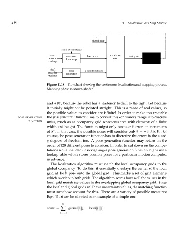
global map 11 Localization and Map Making

for n observations
raw construct local map match and best pose integrate
sensor local map score local into
readings global map

shaft pose k possible poses
encoder generation
readings

Figure 11.18 Flowchart showing the continuous localization and mapping process.
Mapping phase is shown shaded.

and +10 , because the robot has a tendency to drift to the right and because
it initially might not be pointed straight. This is a range of real values, so
the possible values to consider are infinite! In order to make this tractable
POSE GENERATION the pose generation function has to convert this continuous range into discrete
FUNCTION units, much as an occupancy grid represents area with elements of a finite
width and height. The function might only consider errors in increments

of 5 . In that case, the possible poses will consider only = 5; 0; 5; 10 .Of
course, the pose generation function has to discretize the errors in the x and
y degrees of freedom too. A pose generation function may return on the
order of 128 different poses to consider. In order to cut down on the compu-
tations while the robot is navigating, a pose generation function might use a
lookup table which stores possible poses for a particular motion computed
in advance.
The localization algorithm must match the local occupancy grids to the
global occupancy. To do this, it essentially overlays the center of the local
grid at the k pose onto the global grid. This marks a set of grid elements
which overlap in both grids. The algorithm scores how well the values in the
local grid match the values in the overlapping global occupancy grid. Since
the local and global grids will have uncertainty values, the matching function
must somehow account for this. There are a variety of possible measures;
Eqn. 11.16 can be adapted as an example of a simple one:

K
X
j
i
][
[
score = jg obal [i][ j] l o c a l]j
l
k=i;j