Page 170 - Introduction to Autonomous Mobile Robots

Perception

x = (ρ , θ ) 155
i
i
i
d i
r
α

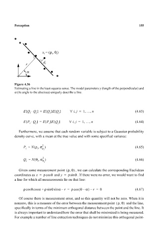
Figure 4.36
Estimating a line in the least-squares sense. The model parameters y (length of the perpendicular) and
α (its angle to the abscissa) uniquely describe a line.

E Q Q ] = E Q ]E Q ] ∀ i j = 1 … n (4.63)
⋅
[
,
,
,
[
[
i
j
i
j
,
,
E P Q ] = E P[]E Q[ ] ∀ i j = 1 … n (4.64)
,
[
⋅
i j i j
Furthermore, we assume that each random variable is subject to a Gaussian probability
density curve, with a mean at the true value and with some specified variance:
P i ~ N ρ σ,( i 2 ρ ) (4.65)
i
Q i ~ N θ σ,( i 2 θ ) (4.66)
i
Given some measurement point ρθ,( ) , we can calculate the corresponding Euclidean
coordinates as x = ρcos θ and y = ρsin θ . If there were no error, we would want to find
a line for which all measurements lie on that line:
α
α
θ
θ
–
ρcos cos + ρsin sin – r = ρcos ( θ α) – r = 0 (4.67)
Of course there is measurement error, and so this quantity will not be zero. When it is
nonzero, this is a measure of the error between the measurement point ρθ,( ) and the line,
specifically in terms of the minimum orthogonal distance between the point and the line. It
is always important to understand how the error that shall be minimized is being measured.
For example a number of line extraction techniques do not minimize this orthogonal point-