Page 175 - Introduction to Autonomous Mobile Robots

160

a) Image Space b) Model Space Chapter 4
β =r [m]
1

β =α [rad]
0
A set of n neighboring points Evidence accumulation in the model space
f
of the image space → Clusters of normally distributed vectors

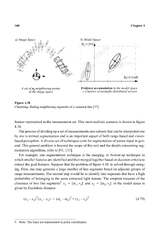
Figure 4.38
Clustering: finding neighboring segments of a common line [37].

feature represented in the measurement set. This more realistic scenario is shown in figure
4.38.
The process of dividing up a set of measurements into subsets that can be interpreted one
by one is termed segmentation and is an important aspect of both range-based and vision-
based perception. A diverse set of techniques exist for segmentation of sensor input in gen-
eral. This general problem is beyond the scope of this text and for details concerning seg-
mentation algorithms, refer to [91, 131].
For example, one segmentation technique is the merging, or bottom-up technique in
which smaller features are identified and then merged together based on decision criteria to
extract the goal features. Suppose that the problem of figure 4.38. is solved through merg-
ing. First, one may generate a large number of line segments based on adjacent groups of
range measurements. The second step would be to identify line segments that have a high
probability of belonging to the same extracted light feature. The simplest measure of the
5
,
,
closeness of two line segments x = [ α r ] and x = [ α r ] in the model space is
1
2
2
2
1
1
given by Euclidean distance:
( x – x ) x – x ) = ( α – α ) + ( r – r ) 2 (4.79)
T
2
(
1 2 1 2 1 2 1 2
5. Note: The lines are represented in polar coordinates.