Page 165 - Introduction to Autonomous Mobile Robots

150

Y Chapter 4

µ + σ y fx()
y
µ
y
µ – σ y
y

X
µ – σ µ µ + σ
x x x x x
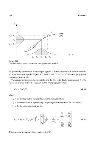
Figure 4.33
One-dimensional case of a nonlinear error propagation problem.

the probability distribution of the output signals Y if they depend with known functions
i
f upon the input signals? Figure 4.33 depicts the 1D version of this error propagation
i
problem as an example.
The general solution can be generated using the first order Taylor expansion of f . The
i
output covariance matrix C is given by the error propagation law:
Y
T
C = F C F X (4.60)
X
X
Y
where
C X = covariance matrix representing the input uncertainties;
C = covariance matrix representing the propagated uncertainties for the outputs;
Y
F is the Jacobian matrix defined as
x
f ∂ f ∂
1
1
-------- … --------
f ∂ X ∂ X
T 1 ∂ ∂ 1 n
F = ∇ f = ∇ ⋅ fX() T = : ∂ X … ∂ X = : … : . (4.61)
X
X
f 1 n f ∂ f ∂
m m m
-------- … --------
∂ X 1 ∂ X n
This is also the transpose of the gradient of fX() .