Page 163 - Introduction to Autonomous Mobile Robots

148

µ) 
2
x –
1  ( Chapter 4
fx() = -------------- exp –  ------------------- 
2
σ 2π  2σ 
68.26%
95.44%
99.72%
-3σ -2σ -σ σ 2σ 3σ

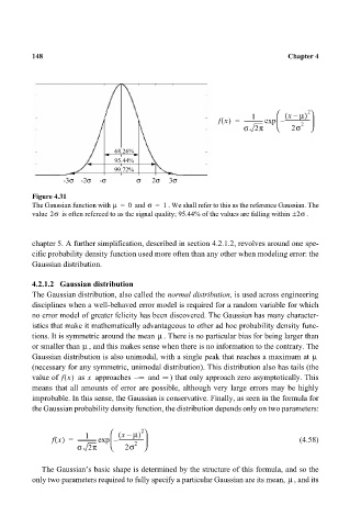
Figure 4.31
The Gaussian function with µ = 0 and σ = 1 . We shall refer to this as the reference Gaussian. The
value 2σ is often refereed to as the signal quality; 95.44% of the values are falling within 2±σ .

chapter 5. A further simplification, described in section 4.2.1.2, revolves around one spe-
cific probability density function used more often than any other when modeling error: the
Gaussian distribution.

4.2.1.2 Gaussian distribution
The Gaussian distribution, also called the normal distribution, is used across engineering
disciplines when a well-behaved error model is required for a random variable for which
no error model of greater felicity has been discovered. The Gaussian has many character-
istics that make it mathematically advantageous to other ad hoc probability density func-
µ
tions. It is symmetric around the mean . There is no particular bias for being larger than
µ
or smaller than , and this makes sense when there is no information to the contrary. The
Gaussian distribution is also unimodal, with a single peak that reaches a maximum at µ
(necessary for any symmetric, unimodal distribution). This distribution also has tails (the
value of fx() as approaches ∞– and ∞ ) that only approach zero asymptotically. This
x
means that all amounts of error are possible, although very large errors may be highly
improbable. In this sense, the Gaussian is conservative. Finally, as seen in the formula for
the Gaussian probability density function, the distribution depends only on two parameters:

 ( µ) 
2
1 x –
fx() = -------------- exp –  -------------------  (4.58)
2
σ 2π  2σ 
The Gaussian’s basic shape is determined by the structure of this formula, and so the
µ
only two parameters required to fully specify a particular Gaussian are its mean, , and its