Page 164 - Introduction to Autonomous Mobile Robots

Perception

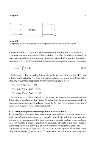
X 1 Y 1 149
… …
X i System Y i
… …
X Y
n m

Figure 4.32
Error propagation in a multiple-input multi-output system with n inputs and m outputs.

σ
standard deviation, . Figure 4.31 shows the Gaussian function with µ = 0 and σ = . 1
X
Suppose that a random variable is modeled as a Gaussian. How does one identify the
µ
chance that the value of is within one standard deviation of ? In practice, this requires
X
integration of fx() , the Gaussian function to compute the area under a portion of the curve:
σ
d
Area = ∫ f x() x (4.59)
– σ
Unfortunately, there is no closed-form solution for the integral in equation (4.59), and
so the common technique is to use a Gaussian cumulative probability table. Using such a
table, one can compute the probability for various value ranges of :
X
[
P µ – σ < X ≤ µ + σ] = 0.68 ;
[
P µ – 2σ < X ≤ µ + 2σ] = 0.95 ;
[
P µ – 3σ < X ≤ µ + 3σ] = 0.997 .
X
For example, 95% of the values for fall within two standard deviations of its mean.
This applies to any Gaussian distribution. As is clear from the above progression, under the
Gaussian assumption, once bounds are relaxed to 3σ , the overwhelming proportion of
values (and, therefore, probability) is subsumed.

4.2.2 Error propagation: combining uncertain measurements
The probability mechanisms above may be used to describe the errors associated with a
single sensor’s attempts to measure a real-world value. But in mobile robotics, one often
uses a series of measurements, all of them uncertain, to extract a single environmental mea-
sure. For example, a series of uncertain measurements of single points can be fused to
extract the position of a line (e.g., a hallway wall) in the environment (figure 4.36).
n
Consider the system in figure 4.32, where X are input signals with a known proba-
i
bility distribution and Y are m outputs. The question of interest is: what can we say about
i