Page 161 - Introduction to Autonomous Mobile Robots

146

Probability Density f(x) Chapter 4

Area = 1

x
0 Mean µ
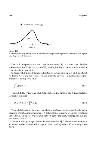
Figure 4.30
A sample probability density function, showing a single probability peak (i.e., unimodal) with asymp-
totic drops in both directions.

From this perspective, the true value is represented by a random (and therefore
unknown) variable . We use a probability density function to characterize the statistical
X
properties of the value of .
X
In figure 4.30, the density function identifies for each possible value of a probabil-
X
x
ity density fx() along the -axis. The area under the curve is 1, indicating the complete
y
X
chance of having some value:
∫ ∞ fx() x = 1 (4.51)
d
– ∞
The probability of the value of falling between two limits and is computed as
a
X
b
the bounded integral:
[
P a < X ≤ b] = ∫ b fx() x (4.52)
d
a
The probability density function is a useful way to characterize the possible values of X
X
because it not only captures the range of but also the comparative probability of different
values for . Using fx() we can quantitatively define the mean, variance, and standard
X
deviation as follows.
The mean value is equivalent to the expected value EX[] if we were to measure X
µ
an infinite number of times and average all of the resulting values. We can easily define
EX[] :