Page 156 - Introduction to Autonomous Mobile Robots

141
Perception
2
2
d
d
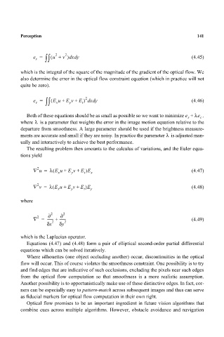
e = ∫ ∫ ( u + v ) x y (4.45)
s
which is the integral of the square of the magnitude of the gradient of the optical flow. We
also determine the error in the optical flow constraint equation (which in practice will not
quite be zero).
2
d
e = ∫ ∫ ( E u + E v + E ) x y (4.46)
d
x
y
t
c
Both of these equations should be as small as possible so we want to minimize e + λe c ,
s
λ
where is a parameter that weights the error in the image motion equation relative to the
departure from smoothness. A large parameter should be used if the brightness measure-
λ
ments are accurate and small if they are noisy. In practice the parameter is adjusted man-
ually and interactively to achieve the best performance.
The resulting problem then amounts to the calculus of variations, and the Euler equa-
tions yield
2
(
∇ u = λ E u + E v + E )E (4.47)
x y t x
2
(
∇ v = λ E u + E v + E )E y (4.48)
x
t
y
where
∂ 2 ∂ 2
2
∇ = ------- + ------- 2 (4.49)
2
x δ y δ
which is the Laplacian operator.
Equations (4.47) and (4.48) form a pair of elliptical second-order partial differential
equations which can be solved iteratively.
Where silhouettes (one object occluding another) occur, discontinuities in the optical
flow will occur. This of course violates the smoothness constraint. One possibility is to try
and find edges that are indicative of such occlusions, excluding the pixels near such edges
from the optical flow computation so that smoothness is a more realistic assumption.
Another possibility is to opportunistically make use of these distinctive edges. In fact, cor-
ners can be especially easy to pattern-match across subsequent images and thus can serve
as fiducial markers for optical flow computation in their own right.
Optical flow promises to be an important ingredient in future vision algorithms that
combine cues across multiple algorithms. However, obstacle avoidance and navigation