Page 155 - Introduction to Autonomous Mobile Robots

140

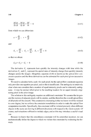
∂ E x ∂ E y ∂ E Chapter 4
d
d
----------- + ----------- + ------ = 0 (4.41)
x ∂ d t y ∂ d t t ∂
from which we can abbreviate

x d y d
u = ----- ; v = ----- (4.42)
t d t d
and

∂ E ∂ E ∂ E
E = ------ ; E = ------ ; E = ------ = 0 (4.43)
x x ∂ y y ∂ t t ∂

so that we obtain

E u + E v + E = 0 (4.44)
x y t
The derivative E represents how quickly the intensity changes with time while the
t
derivatives E and E represent the spatial rates of intensity change (how quickly intensity
x y
changes across the image). Altogether, equation (4.44) is known as the optical flow con-
straint equation and the three derivatives can be estimated for each pixel given successive
images.
We need to calculate both u and v for each pixel, but the optical flow constraint equation
only provides one equation per pixel, and so this is insufficient. The ambiguity is intuitively
clear when one considers that a number of equal-intensity pixels can be inherently ambig-
uous – it may be unclear which pixel is the resulting location for an equal-intensity origi-
nating pixel in the prior image.
The solution to this ambiguity requires an additional constraint. We assume that in gen-
eral the motion of adjacent pixels will be similar, and that therefore the overall optical flow
of all pixels will be smooth. This constraint is interesting in that we know it will be violated
to some degree, but we enforce the constraint nonetheless in order to make the optical flow
computation tractable. Specifically, this constraint will be violated precisely when different
objects in the scene are moving in different directions with respect to the vision system. Of
course, such situations will tend to include edges, and so this may introduce a useful visual
cue.
Because we know that this smoothness constraint will be somewhat incorrect, we can
mathematically define the degree to which we violate this constraint by evaluating the for-
mula