Page 154 - Introduction to Autonomous Mobile Robots

Perception

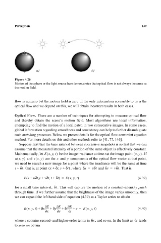
a) b) 139

Figure 4.26
Motion of the sphere or the light source here demonstrates that optical flow is not always the same as
the motion field.

flow is nonzero but the motion field is zero. If the only information accessible to us is the
optical flow and we depend on this, we will obtain incorrect results in both cases.

Optical Flow. There are a number of techniques for attempting to measure optical flow
and thereby obtain the scene’s motion field. Most algorithms use local information,
attempting to find the motion of a local patch in two consecutive images. In some cases,
global information regarding smoothness and consistency can help to further disambiguate
such matching processes. Below we present details for the optical flow constraint equation
method. For more details on this and other methods refer to [41, 77, 146].
Suppose first that the time interval between successive snapshots is so fast that we can
assume that the measured intensity of a portion of the same object is effectively constant.
Mathematically, let E xy t,,( ) be the image irradiance at time t at the image point xy,( ) . If
ux y,( ) and vx y,( ) are the and components of the optical flow vector at that point,
y
x
we need to search a new image for a point where the irradiance will be the same at time
δ
,
t + t δ , that is, at point x +( t δ y + t δ ) , where xδ = u tδ and yδ = vt . That is,
δ
δ
(
,,
,
,
(
E x + u t y + v t t + t δ ) = E xyt) (4.39)
for a small time interval, tδ . This will capture the motion of a constant-intensity patch
through time. If we further assume that the brightness of the image varies smoothly, then
we can expand the left hand side of equation (4.39) as a Taylor series to obtain
∂
∂
∂
E
E
E
(
,,
,,
(
Exyt) + δ x------ + δ y------ + δ t------ + e = Exyt) (4.40)
x ∂ y ∂ t ∂
where e contains second- and higher-order terms in xδ , and so on. In the limit as tδ tends
to zero we obtain