Page 149 - Introduction to Autonomous Mobile Robots

Chapter 4
134
So the Laplacian represents the second derivative of the image, and is computed along
both axes. Such a transformation, called a convolution, must be computed over the discrete
space of image pixel values, and therefore an approximation of equation (4.35) is required
for application:

L = P ⊗ I (4.36)

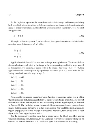
We depict a discrete operator , called a kernel, that approximates the second derivative
P
operation along both axes as a 3 x 3 table:

010
–
14 1 (4.37)
010

Application of the kernel to convolve an image is straightforward. The kernel defines
P
the contribution of each pixel in the image to the corresponding pixel in the target as well
as its neighbors. For example, if a pixel (5,5) in the image has value I 55,( ) = 10 , then
I
application of the kernel depicted by equation (4.37) causes pixel I 5 5,( ) to make the fol-
L
lowing contributions to the target image :
L 5 5,( ) += -40;
L 4 5,( ) += 10;
L 6 5,( ) += 10;
L 5 4,( ) += 10;

L 5 6,( ) += 10.

Now consider the graphic example of a step function, representing a pixel row in which
the intensities are dark, then suddenly there is a jump to very bright intensities. The second
derivative will have a sharp positive peak followed by a sharp negative peak, as depicted
in figure 4.23. The Laplacian is used because of this extreme sensitivity to changes in the
image. But the second derivative is in fact oversensitive. We would like the Laplacian to
trigger large peaks due to real changes in the scene’s intensities, but we would like to keep
signal noise from triggering false peaks.
For the purpose of removing noise due to sensor error, the ZLoG algorithm applies
Gaussian smoothing first, then executes the Laplacian convolution. Such smoothing can be
effected via convolution with a 3 × 3 table that approximates Gaussian smoothing: