Page 275 - Introduction to Autonomous Mobile Robots

260

y θ 2 Chapter 6
2
1
θ 2
θ 1

3
4
θ
x 1
a) b)
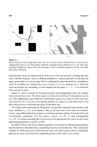
Figure 6.1
Physical space (a) and configuration space (b): (a) A two-link planar robot arm has to move from the
configuration start to end. The motion is thereby constraint by the obstacles 1 to 4. (b) The corre-
sponding configuration space shows the free space in joint coordinates (angle θ and θ ) and a path
1
2
that achieves the goal.
physical space from the initial position of the arm to the goal position, avoiding all colli-
sions with the obstacles. This is a difficult problem to visualize and solve in the physical
space, particularly as grows large. But in configuration space the problem is straightfor-
k
ward. If we define the configuration space obstacle O as the subspace of C where the
robot arm bumps into something, we can compute the free space F = C – O in which the
robot can move safely.
Figure 6.1 shows a picture of the physical space and configuration space for a planar
robot arm with two links. The robot’s goal is to move its end effector from position start to
end. The configuration space depicted is 2D because each of two joints can have any posi-
tion from 0 to 2π . It is easy to see that the solution in C-space is a line from start to end
that remains always within the free space of the robot arm.
For mobile robots operating on flat ground, we generally represent robot position with
three variables xy θ,,( ) , as in chapter 3. But, as we have seen, most robots are nonholo-
nomic, using differential-drive systems or Ackerman steered systems. For such robots, the
nonholonomic constraints limit the robot’s velocity x y θ,,( · · · ) in each configuration
( xy θ) . For details regarding the construction of the appropriate free space to solve such
,,
path-planning problems, see [21, p. 405].
In mobile robotics, the most common approach is to assume for path-planning purposes
that the robot is in fact holonomic, simplifying the process tremendously. This is especially
common for differential-drive robots because they can rotate in place and so a holonomic
path can be easily mimicked if the rotational position of the robot is not critical.