Page 280 - Introduction to Autonomous Mobile Robots

Planning and Navigation

start 265
7 8 17

9 10

5
1 6 18

14
4 15
2
3
16
11 12 13
goal

7 8 9 10 17

1 5 6 14 18

2 3 4 11 12 13 15 16
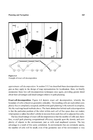
Figure 6.4
Example of exact cell decomposition.

approximate cell decomposition. In section 5.5.2 we described these decomposition strate-
gies as they apply to the design of map representation for localization. Here, we briefly
summarize these two cell decomposition techniques once again, providing greater detail
about their advantages and disadvantages relative to path planning.

Exact cell decomposition. Figure 6.4 depicts exact cell decomposition, whereby the
boundary of cells is based on geometric criticality. The resulting cells are each either com-
pletely free or completely occupied, and therefore path planning in the network is complete,
like the road map based methods above. The basic abstraction behind such a decomposition
is that the particular position of the robot within each cell of free space does not matter;
what matters is rather the robot’s ability to traverse from each free cell to adjacent free cells.
The key disadvantage of exact cell decomposition is that the number of cells and, there-
fore, overall path planning computational efficiency depends upon the density and com-
plexity of objects in the environment, just as with road mapbased systems. The key
advantage is a result of this same correlation. In environments that are extremely sparse,
the number of cells will be small, even if the geometric size of the environment is very