Page 286 - Introduction to Autonomous Mobile Robots

Planning and Navigation

a) Classical Potential 271

Goal

b) Rotation Potential
with parameter β
Goal

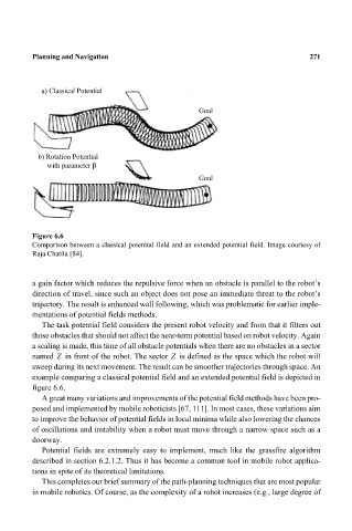
Figure 6.6
Comparison between a classical potential field and an extended potential field. Image courtesy of
Raja Chatila [84].

a gain factor which reduces the repulsive force when an obstacle is parallel to the robot’s
direction of travel, since such an object does not pose an immediate threat to the robot’s
trajectory. The result is enhanced wall following, which was problematic for earlier imple-
mentations of potential fields methods.
The task potential field considers the present robot velocity and from that it filters out
those obstacles that should not affect the near-term potential based on robot velocity. Again
a scaling is made, this time of all obstacle potentials when there are no obstacles in a sector
Z
Z
named in front of the robot. The sector is defined as the space which the robot will
sweep during its next movement. The result can be smoother trajectories through space. An
example comparing a classical potential field and an extended potential field is depicted in
figure 6.6.
A great many variations and improvements of the potential field methods have been pro-
posed and implemented by mobile roboticists [67, 111]. In most cases, these variations aim
to improve the behavior of potential fields in local minima while also lowering the chances
of oscillations and instability when a robot must move through a narrow space such as a
doorway.
Potential fields are extremely easy to implement, much like the grassfire algorithm
described in section 6.2.1.2. Thus it has become a common tool in mobile robot applica-
tions in spite of its theoretical limitations.
This completes our brief summary of the path-planning techniques that are most popular
in mobile robotics. Of course, as the complexity of a robot increases (e.g., large degree of