Page 288 - Introduction to Autonomous Mobile Robots

Planning and Navigation

goal 273

L2

H1 L1 H2

start

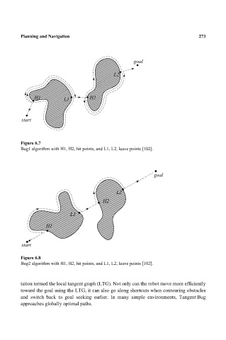
Figure 6.7
Bug1 algorithm with H1, H2, hit points, and L1, L2, leave points [102].

goal

L2
H2

L1
H1

start

Figure 6.8
Bug2 algorithm with H1, H2, hit points, and L1, L2, leave points [102].

tation termed the local tangent graph (LTG). Not only can the robot move more efficiently
toward the goal using the LTG, it can also go along shortcuts when contouring obstacles
and switch back to goal seeking earlier. In many simple environments, Tangent Bug
approaches globally optimal paths.